The Earth, wired.
Four drawings of one habit of mind: read any system as stores, couplings, and the loops between them. The wiring of the whole Earth, that same Earth as a control loop, one tipping element reaching across the planet, and a single place solved as a second-order system. The pictures behind The Lens.
The whole system, wired.
Every sphere drawn as a store; every arrow a coupling that carries energy, water, carbon or sediment from one to the next.
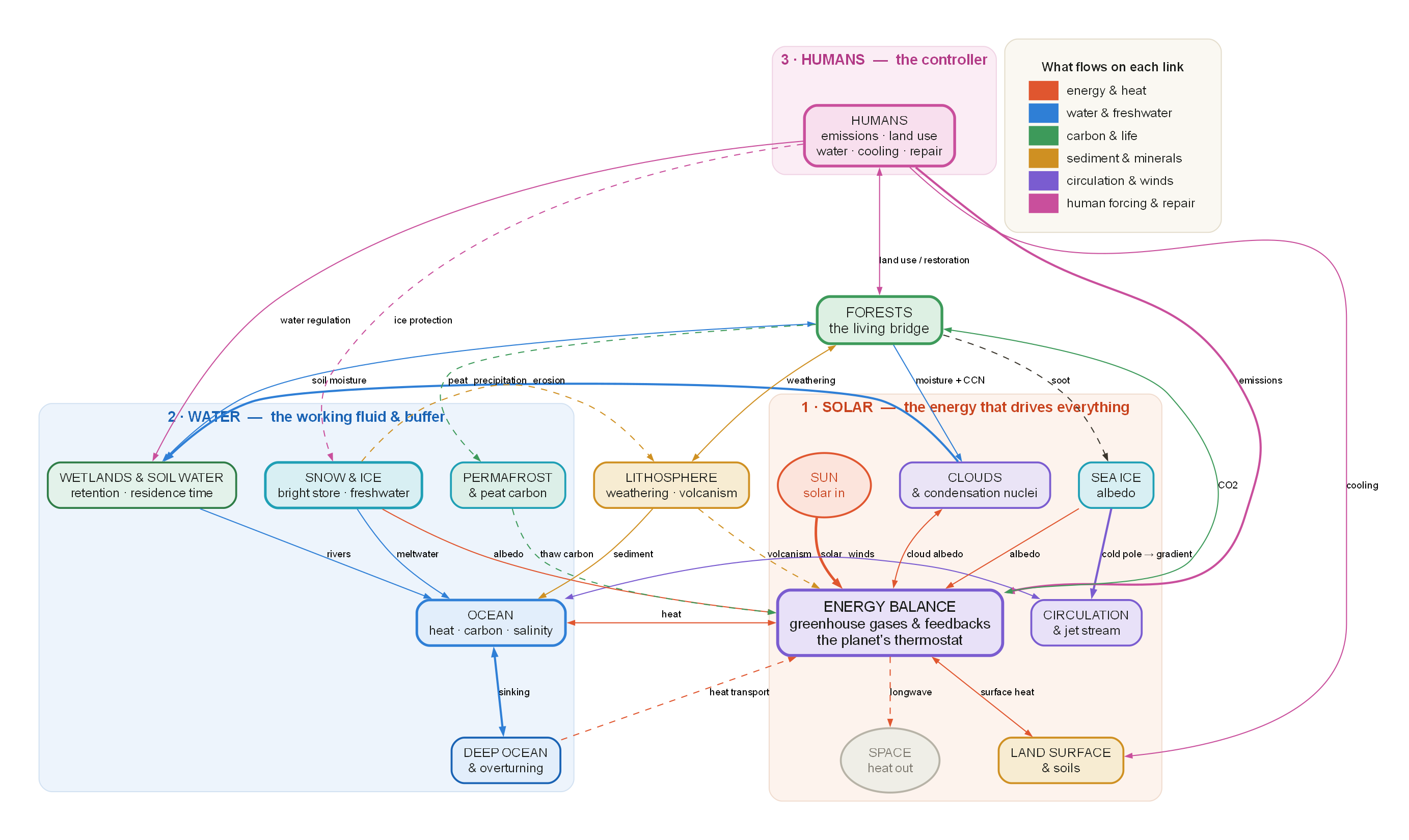
This is the map before any equation. Each box is a store that holds something and passes it on; each arrow is a coupling, coloured by the currency it carries.
The point is never the parts on their own. It is the wiring between them: the couplings that let a change in one sphere become a change in all the others. Read the wiring and you can already see where a failure will travel, and where a repair could begin.
The same Earth, as a feedback loop.
Redraw the couplings as a control diagram and the climate becomes a second-order system: a balance, its stores, the water cycle's phase changes, and the loops that stabilise or run away.
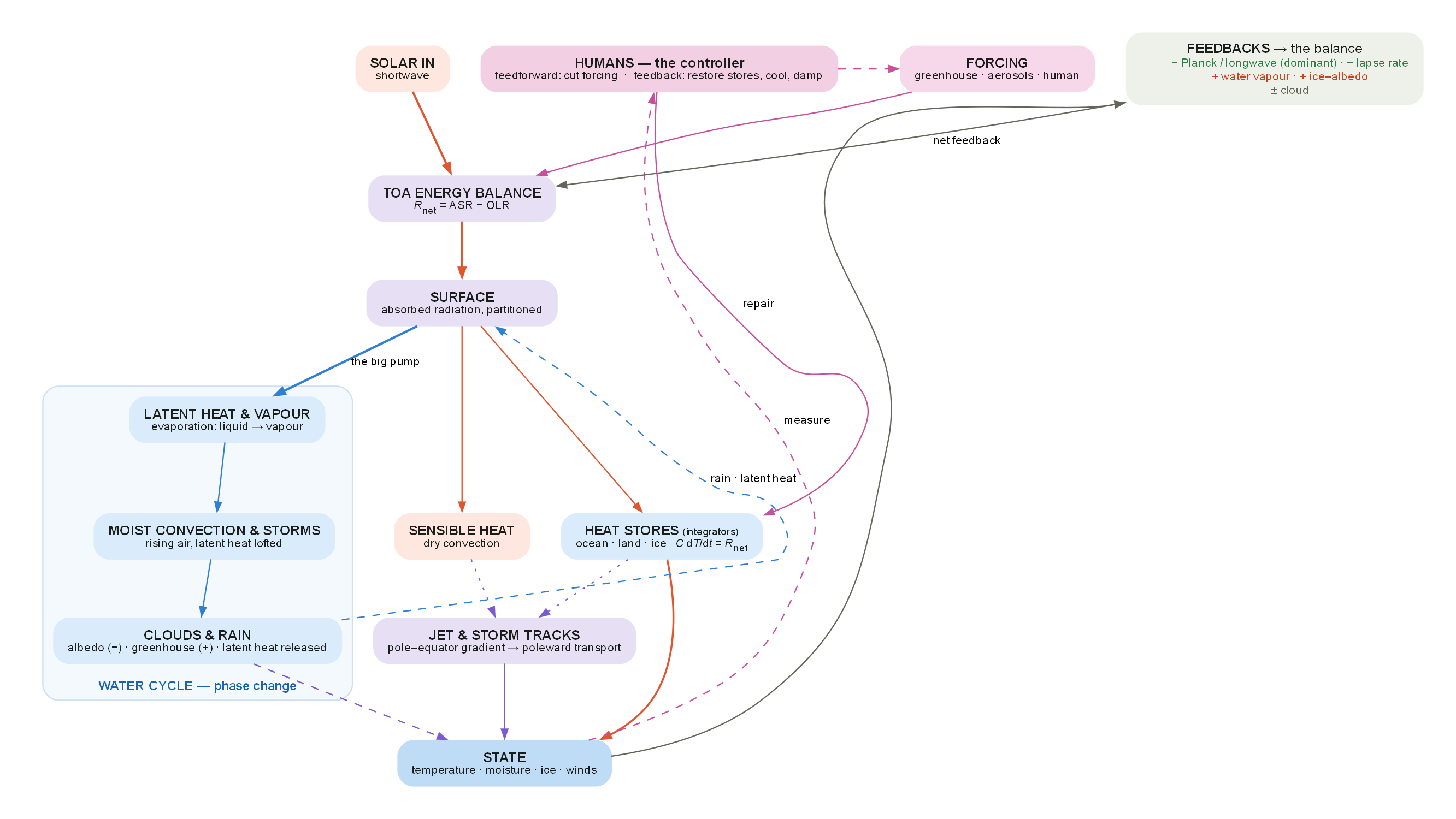
The same couplings, redrawn the way control engineering draws a machine. Sunlight and forcing enter a balance; the surface partitions the energy into stores and into the water cycle, whose phase changes do most of the real work.
Every arrow that returns is a loop. Some pull the state back toward balance; some push it further out. The human sits at the bottom as a controller with two moves: cut the forcing, and repair the stores.
One tipping element, across the planet.
Put the couplings on a real map and you can trace how a change in one place reaches every other: the Arctic to the Amazon, dams to the AMOC.
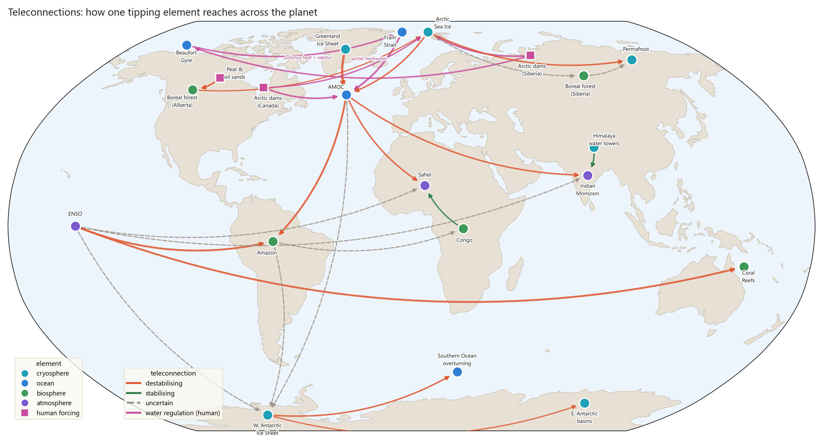
Coupling is not only local. A map of the tipping elements, wired by their real teleconnections, shows a change in one place arriving, weeks or decades later, somewhere else entirely.
The magenta layer is the part that standard accounting misses: subarctic dams whose winter freshwater preconditions the AMOC, and whose open-water plumes force the Arctic thermal state. A distinct, human, water-regulation forcing, sitting beside the natural ones.
One place, as a second-order system.
Zoom to a single patch and the same lens becomes exact: mass, spring, damper, and a pole-zero map that shows how near the loop is to opening.
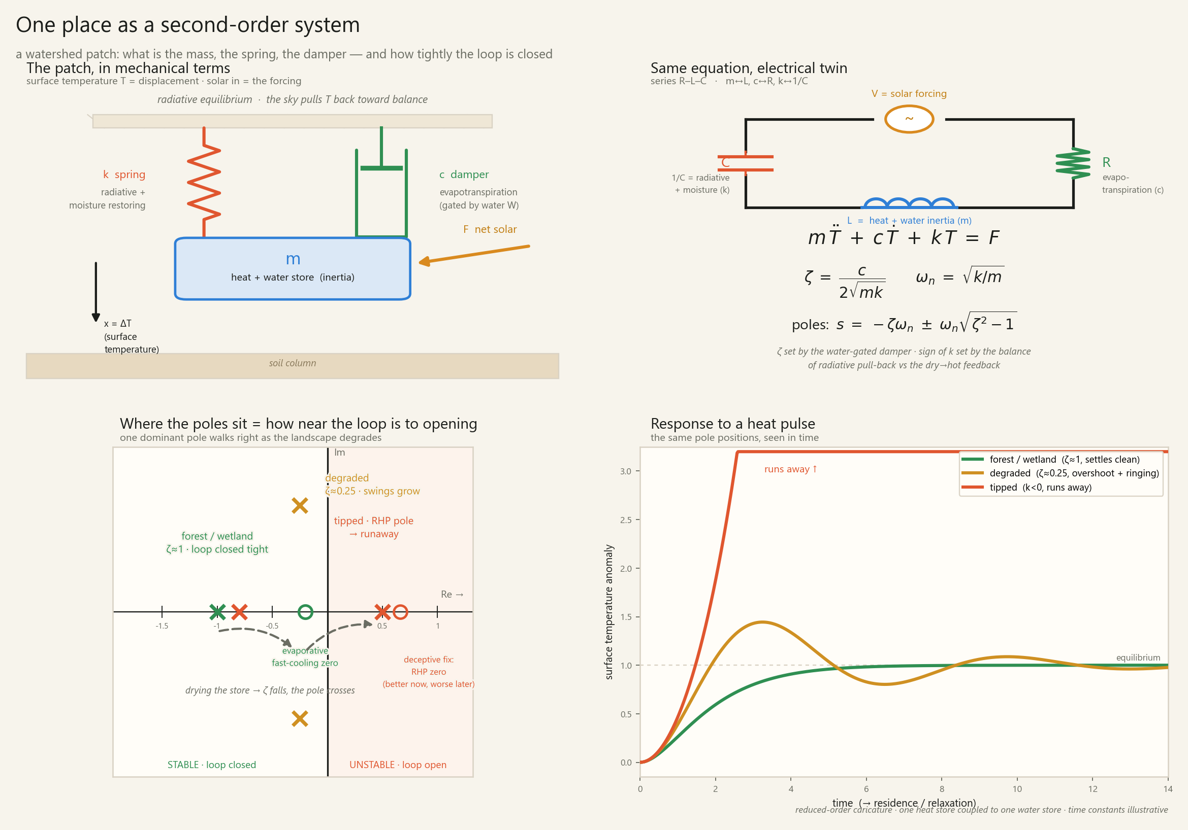
Down at one place the wiring becomes a single equation. The heat-and-water store is the mass; the radiative pull-back is the spring; evapotranspiration, gated by the water the land still holds, is the damper.
Where the poles sit is the whole story. A living, well-watered landscape keeps the loop closed tight. Dry the store and the damping falls, the swings grow, and one pole walks toward the imaginary axis. Cross it and the loop is open: runaway.
The same lens on a real place: Gatún.
The generic model, pinned to the Panama Canal's reservoir with its measured timescales. The poles land on the one-year residence and three-month turnover of the real lake.
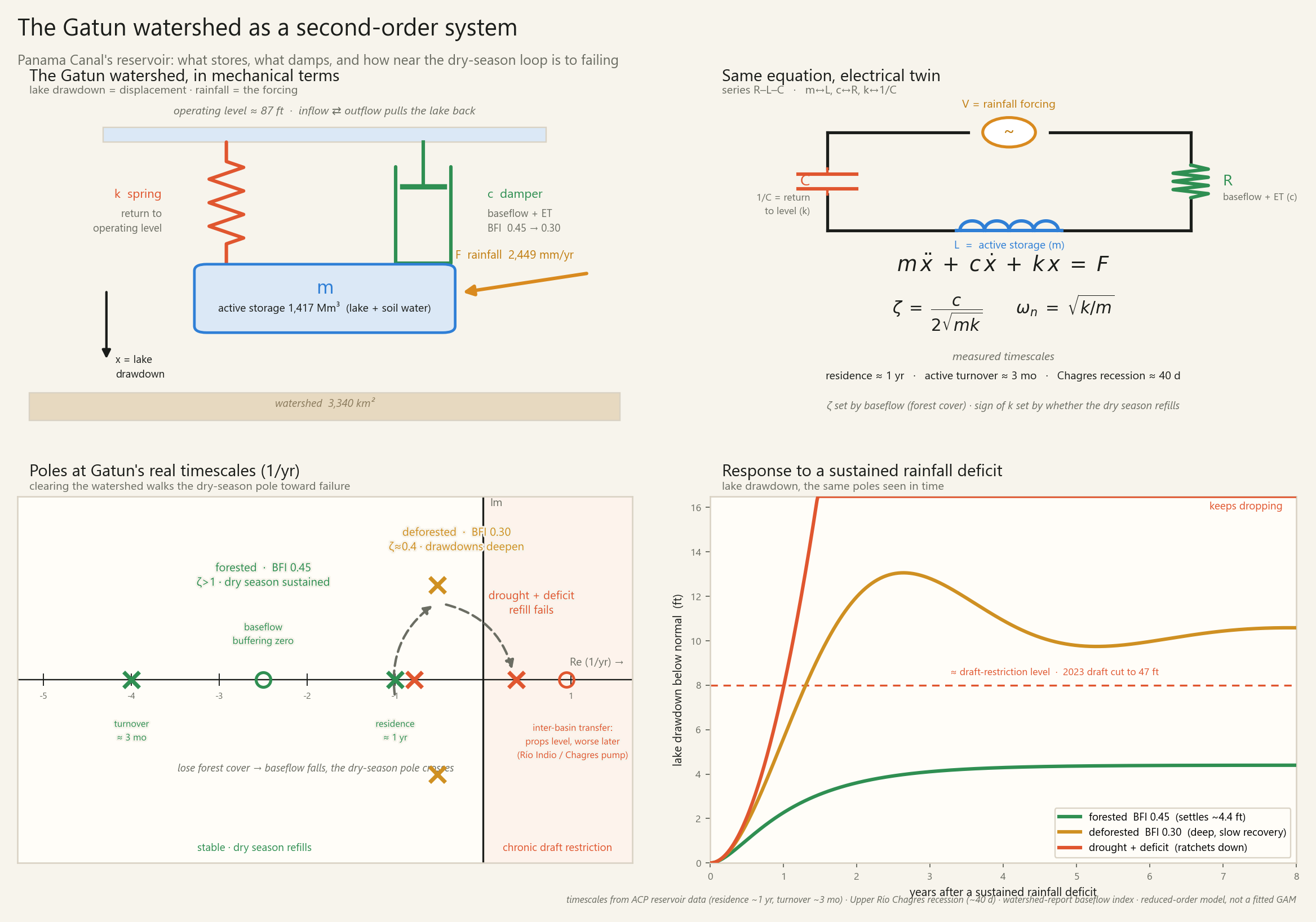
The abstraction earns its keep only if it survives contact with a real basin. Here the forested poles land where the measurements say they should: one at the lake's one-year residence, one at its three-month active-storage turnover.
Clearing the catchment lowers the baseflow index, the damping falls, and the dry-season pole slides toward failure: the draft restrictions that now stop ships in a drought year. The picture is honest about its limits, but the mechanism it shows is the modifiable one.
These are the pictures. To learn the six words that make them read the way an engineer reads a circuit, start with The Lens. To watch the same lens turned on real places, read the case studies.